Activity #9 – Basic Video Processing

Welcome to the last activity blog post for the Applied Physics 186 Experience. So far, we have been doing a lot of single image processing: from digital scanning to morphological operations. And yes, we have managed to process a lot of images. It is now time to integrate what we have learned and do video processing.

A video consists of strings of different images that are in sequence with one another that are shown in rapid succession. Through videos, one can demonstrate motion by the rapid succession of images that depict kinematic processes such as people running, objects falling or even the growth of bacteria. A digital video has its own frame rate for image capturing, which will tell the number of frames or images per second the video shows (frames per second = fps). Its inverse is then the time interval between two succeeding images. By combining then what we have learned from single image processing towards videos, we can then analyze time-dependent parameters using images such as the rate at which an object falls. [1]

In this activity, we investigate terminal velocity from free-fall in air. Classical mechanics would tell us that an object falling at a certain height would fall with an acceleration of g = 9.8 m/s² if air resistance is neglected. This means that if an object would continuously fall without air resistance, the object’s velocity would increase infinitely. However, this is not true when air resistance is not neglected. As we know, this air resistance acts as a drag force which counters the relative motion of the object through air. This drag force is directly proportional to the velocity of a particle. A free-falling particle would then reach into a point where the drag force becomes equal to the force of gravity, in which at this state, the velocity of the particle would become constant. This constant velocity is called “Terminal Velocity” by brave skydivers.

To investigate terminal velocity in our dearest NIP building, me and my partner John Kevin Sanchez worked on an experiment involving free-fall and air resistance. We allowed an upside-down umbrella (thanks to Mario for bravely sharing us his umbrella) to free-fall from the 4th floor of the NIP building towards the first floor. Since the mass and area of the umbrella that is in contact with the air  is sufficient for air drag to take effect, we expect the umbrella to reach terminal velocity. However, we don’t have the right tools to physically measure the velocity of the falling umbrella. Luckily, there’s video processing to the rescue!

To do the actual set-up, we searched for the best place to take a video from the process, which would be the second floor of the building. JK would let the umbrella fall, and I am the one who’s going to catch it. We give our thanks for our professor, Ms. Soriano, for allowing us to borrow her Olympus DSLR camera, and for helping us take the video of the experiment. Here’s a GIF file of a clip from the video, which depicts the fall of the umbrella.

Figure 1. GIF file of a clip from the umbrella experiment video. Total running time in the clip is 3.87 seconds. Frame rate of the video camera is 59 fps while the frame rate used for video processing is 15 fps.

The GIF is a slower than the actual video, in which the part where the umbrella falls is about 4 seconds. I, for one, could see that the umbrella had been falling at an almost constant velocity since the start of the fall. But taking my judgement aside, let us move on with basic video processing. Before we move on processing our video, one important thing to note is that the type of file the video would have will depend on the camera and program used. Therefore, one should convert the video into an appropriate format, which will enable your program to extract the frames associated with the video. In the camera used, the video is saved into an MTS file, which is a format used for most modern digital cameras. One good freeware that can extract frames from a video is VirtualDub. However, this program can only process specific video formats, and at a reduced time frame only, unless one could buy its premium offer. For the video converter, the STOIK Video Converter is also a freeware that could convert most of video file types into another. Similar to the VirtualDub, one is limited to specific file types unless you buy their stuff. Money changes everything. Another cool stuff is Free Video to JPG converter by DVDVideoSoft. In this activity, I used Adobe Photoshop to manipulate the video and extract its image sequences frame by frame. I also used it to convert the video into a GIF file.

The raw video acquired from the camera is set to 59 fps. As gamers would know, 60 fps is the benchmark value for video frame rate for the best gaming experience. However, this value is a bit big for basic video processing, since this means that for every 1 second, we are to process about 59 images. So in this case, I will be taking off some of the images, and limit the frame rate to 15 fps. The time step for each image would then be 1/15 or 0.0667 seconds. One must be also careful in choosing the frame rate for video processing, as this value will dictate the timestep essential in modelling kinematic variables. Since the clip’s running time is 3.87 secodns, a 0.0667-s timestep is sufficient for modelling. A higher fps would lead to the most accurate model, but would take a lot of processing power to finish the coding in a small span of time.

What would we want now is to determine the umbrella’s speed from the video itself. To do that, we have to find a way to treat the umbrella as a particle and approximate its position from the images. One way is to do an image segmentation to extract the shape of the umbrella, then calculate its centroid. To do image segmentation, one has to extract a region of interest (ROI) that has the same color brightness and hue with the umbrella. Fortunately, the umbrella has a distinct color relative to the background, and so image segmentation is a bit easier. If you haven’t seen my blog post about image segmentation, then you can always check out my previous post about it. The method I used in segmenting is by doing a joint probability distribution to check pixel membership since Scilab takes a huge time to do histogram backproject, especially for this video, which has a resolution of 1080×1920 pixels.

One drawback from doing a parametric image segmentation is that more pixels will be included as long as its value belongs to the probability distribution. This will then include stray intensities in the segmentation, which will significantly affect the centroid value. We then have to do morphological operations towards the segmented image to clear out these intensities. Since the background is black, we would then have to use OpenImage() to erode these intensities, then dilate the shape of the umbrella to its original form. Here is a GIF file of the segmented video.

Figure 2. Animation for the segmented part of the video. This is for the parametric segmentation.

The segmentation in this part has been rugged, and separation of pixel clusters can be observed. I made improvements by combining both closing and opening morphological operations. I also pushed my laptop to do non-parametric image segmentation, so that I can exploit the quality of the ROI.

Figure 3. Animation for the segmented part of the video. This is for the non-parametric segmentation.

As it is clear from the GIF, the shape of the umbrella has degraded from the starting point towards the end. The logo on the umbrella really takes its toll on the left part of the segmentation. The umbrella has black segments that separates the blue parts, which separates the umbrella into segments. The opening operator could have diminished some of the parts. In addition to that, binary image thresholding was done on the image, so some parts of the umbrella that have a grayscale value would also be cut off. Another aspect would be the tilting of the umbrella as it falls, since this will reduce the blue part. This will then give significant effect to the centroid of the shape, since some of the pixels have been cut off. That is why I picked a smaller timestep to make sure that the movement of the centroid is as small as possible. The centroid is calculated by finding all the coordinates of the white pixels in the shape of the umbrella, and then calculating its mean value.

Time for some plotting! To convert the pixel values to actual distances, we looked for a scaling ratio. Using a long tape measure, we measured the actual distance from the third floor to the second floor, and then used meter-to-pixel ratio calculation to convert the pixel values to distances. A 1 pixel distance in this video is approximately 0.00539 meters. The timestep for each image is then 0.0667 s. And here are the results!

Figure 4. Distance vs Time plot for the free-fall experiment when parametric segmentation is used. Timestep used: 0.0667 seconds.

Figure 5. Distance travelled vs Time graph of the umbrella fall with non-parametric segmentation.

So far so good! The motion has initially  is curved, where in this phase, the umbrella picks up its velocity. After about half a second, the effect of air resistance becomes visible, as the distance growth becomes approximately linear. The curved part refers to initial free-fall motion, where air drag force is still negligible since the velocity of the umbrella is still low. After it has gained enough speed, the air drag begins to counter the force of gravity. A linearly increasing function would then have a constant slope value, where in this case, is the terminal velocity. One then can do differentiation on the graph and obtain a horizontal line in the linear part. The difference between the two segmentations were not that big.

We can then obtain more information about the graph such as drag coefficient and terminal velocity. For the terminal velocity, we do a linear fit in the straight part of the graph. I did this in MS Excel to extract the equation easily.

Figure 6. Linearly-fitted graph of the distance function when parametric segmentation is used.

 

Figure 7. Linearly-fitted graph of the distance function when parametric segmentation is used.

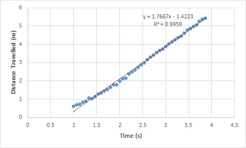
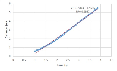
The terminal velocity is then 1.767 m/s from the graph. This is then particularly useful in large-scale experiment measurements involving kinematic motion. This calculation will suffice from now, since I still have to figure out a way to find drag coefficient given the parameters. Moreover, the slope value has about 0.01 m/s difference, which is not that big also.

With that I end the last activity blog post for the course AP 186 – Image Processing. This may be the most tedious of them all since my computer has suffered a lot of backlash from tons of frames and images. For the hardwork and quality, I may as well give myself a 12. Nevertheless, I would say I have developed the skill of handling a large number of files.  This has been a very fruitful semester, since I have learn a lot not only about images, but also the techniques and processes that made digital image processing. I could’ve wished for a longer time, since most of the interesting lessons on image processing such as pattern recognition, neural networks, and shape analysis were left out due to time constraint. This maybe the last blog post for the course, but this will not end the image processing journey. Maybe someday, when I’ve learned something new I would share it, whether it may be about image processing or not.

Acknowledgements: My gratitude to my partner, Mr. John Kevin Sanchez for running up and down in the NIP building just to get the best results, and also for being patient in uploading the video, since my laptop’s hard drive bluntly deleted everything I worked for. My dearest thanks for Ms. Soriano for all the tips, tools, lessons, everything. And also special thanks to Mario Onglao for that magnificent blue umbrella. You and that thing will be forever missed. Selfie time!

“Nothing’s like a good selfie, boys!”

Let’s end this post with a GIF.

References:

[1] M. Soriano, “Activity 9 – Basic Video Processing,” 2015.